Chicago Transit Ridership Panel
Project link: https://github.com/eric-mc2/DNCTransit
This page describes the steps I took to create a panel dataset of ridership across different Chicago transit systems. I did this to practice econometric modeling.
Transit modes and data sources
Included modes
- Train, Bus, Rideshares - from the City of Chicago (used Socrata API and sodapy python package)
- Bikeshares aka Divvy Bikes - from Lyft (used s3fs python package to access public Amazon S3 bucket)
Excluded modes
- Metra commuter rail (public data is available but too coarsely aggregated)
- Pace city-suburb bus link (have not checked availability)
- Walking / Biking (vendored data is available – ie cell phone location data – but would be hard to isolate from other transit modalities)
- Driving (public data is available – ie road segment usage – but haven’t seriously looked yet)
Extra data
- Geographic boundaries - from US Census Bureau (used pygris python package)
- Landmark boundaries - also from City of Chicago
ETL Pipeline
Major steps in processing this data:
- Extract
- Get raw unit-level data (i.e. train stations, bus lines)
- Get raw ridership time series data
- Transform
- Account for schema drift in each data source
- Merge unit info and time series data
- Compute and add covariates for regression
- Merge
- Merge transit modalities at different spatial and time aggregations
- Choose
- Choose best aggregation for regression modeling
ETL Illustration
Some datasets were better organized than others. The easier ones only required:
- selecting spatial and time range to query
- reading data documentation
- figuring out which are the table primary and foreign keys
- light conversion of data and object types
In the simplest of cases, here’s all the code we need to query and arrange a panel:
from src.data.cta import (ChiClient,
                          BUS_ROUTES_TABLE,
                          BUS_RIDERSHIP_TABLE)
from src.data.gis import WORLD_CRS
from shapely.geometry import shape

# Query static info about bus routes
client = ChiClient(60)
bus_routes =  client.get_all(BUS_ROUTES_TABLE, select="the_geom, route, name")
bus_routes = (bus_routes
            .assign(geometry = bus_routes['the_geom'].apply(shape))
            .drop(columns='the_geom')
            .pipe(gpd.GeoDataFrame, crs=WORLD_CRS))

# Query daily rides per route
data_start = "2024-01-01T00:00:00"
data_end = "2024-08-31T23:59:59"
bus_rides = client.get_all(BUS_RIDERSHIP_TABLE,
                            select="route,date,daytype,rides",
                            where=f"date between '{data_start}' and '{data_end}'")

bus_panel = bus_rides.merge(bus_routes, how='left', on='route')
Let’s plot these routes, colored by ridership:
After getting the direct transit data, I coded a few extra features such as census tract and population, which could serve as useful regression controls later on.
import pygris

# CTA routes extend outside chicago into cook cty.
tracts = pygris.tracts(state='IL', county='cook', cb=True, year=2020, cache=False)
tracts = tracts[['GEOID','geometry']]
tracts['GEOID'] = pd.to_numeric(tracts['GEOID'])

def code_tract(gdf, tracts_gdf) -> pd.Series:
    """Spatial join points to census tract"""
    codes = (gdf
            .filter(['geometry'])
            .to_crs(tracts_gdf.crs)
            .sjoin(tracts_gdf, how='left', predicate='within'))
    return pd.concat([gdf, codes['GEOID'].rename('tract'), axis=1])

bus_stops = bus_stops.pipe(code_tract)
Now we know the immediate population served by each bus line.
Since ridership is reported at different levels of granularity for each transit modality, I had to be careful how to spatially aggregate the data. My goal is to test whether local events, such as football games, have a measurable effect on transit. Associating transit stations to points of interest is straightforward – each point is an unambiguous distance away. Associating shapes such as bus routes or census tracts is more ambiguous – do we measure the distance to the closest bus stop or the furthest? The data doesn’t tell us whether riders travel short or far distances along these routes. This ambiguity can create inaccurate regression estimates.
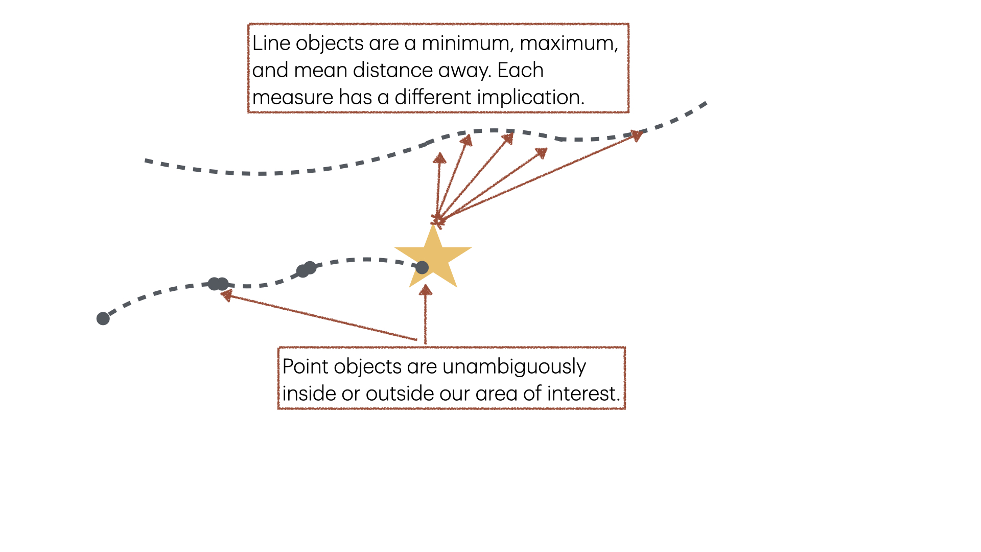
- Train: provides daily boarding counts per station. we do not know where each passenger exited, nor which direction or train route they took.
- Bus: provides daily boardings counts per route. we do not know how this breaks down per bus stop, nor the direction or stop passengers exited at.
- Bike: provides trip-level data: timestamped station pickups and dropoffs per ride.
- Bike: provides trip-level data: timestamped pickup and dropoffs per ride. pickup and dropoff points are anonymized to their containing census tract.
| Modality | Train | Bus | Bike | Uber |
|---|---|---|---|---|
| Time granularity | Daily | Daily | Minute | Minute |
| Direction of travel | No | No | No | No |
| Point of departure | Yes | No | Yes | No |
| Line of departure | Inferred | Yes | No | No |
| Area of departure | Yes | No | Yes | Yes |
| Point of arrival | No | No | Yes | No |
| Line of arrival | Inferred | Yes | No | No |
| Area of arrival | Yes | No | Yes | Yes |
I aggregated three comparable panels:
- Point: train, bike
- Line: train, bus
- Area: train, bike, uber
Special Challenges
Divvy Locations
The divvy historical data spans from 2013 to 2024. Over these years, the published schema has changed several times. This led to annoying, but forgiveable issues to work around:
Batch Size: Some years are published in monthly batches, others quarterly. This isn’t an issue for data modeling, since we just concatenate, but it requires extra logic for properly discovering and enumerating the available data.
Inconsistent column names: Also not an issue for modeling, since I just rename them, but requires manually curating a mapping of {old name -> new name} .
Normalized vs Denormalized: Some years contain data in “database normalized” format with separate stations and rides tables, linked by a common station_id key. Other years only contain a single de-normalized/merged rides table, with station info included.
But the divvy data contained two way worse problems:
Unstable station id’s
In some batches, the station ID is an integer, while in others it is a UUID, representing schema drift. This drift broke the one-to-one property of station IDs: 60% of station IDs were one-to-many: they were associated with up to 4 unique stations.
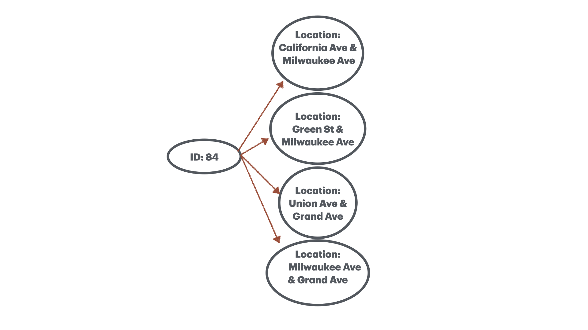
For those not familiar with Chicago streets, these intersections are quite far apart:
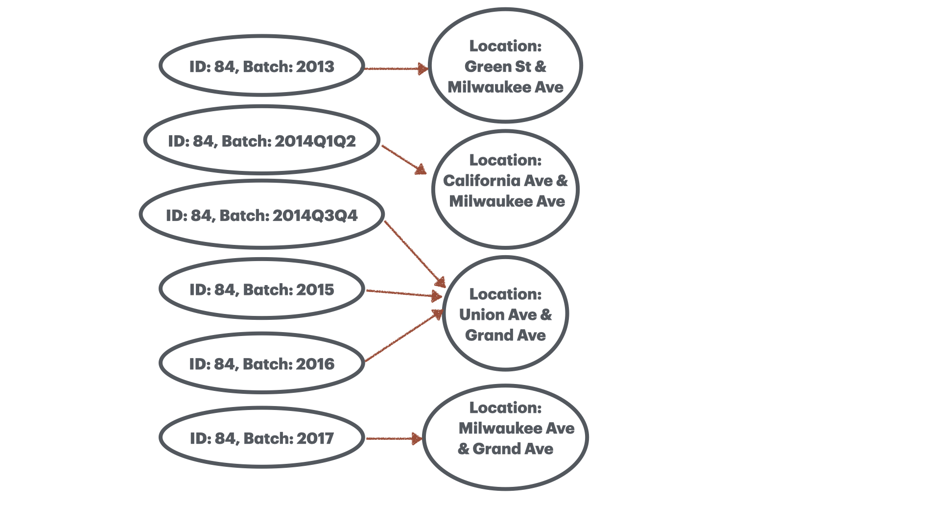
The standard approach to resolving this issue is to create a column labeling each observation with the batch it came from (eg. “2024-Q1”) and use (ID, batch) pairs as the new primary key. Although this fixes the one-to-many issue, it breaks the injective property of station IDs, making them many-to-one!
Unstable station name
Looking at the data this way, perhaps the station name is a sufficient primary key?
Unfortunately, station names were also not always one-to-one. For example, the following locations are all purportedly at Buckingham Fountain:
Similarly, station names were also not always injective.
Imprecise station locations
Recent Divvy historical data batches are published as single denormalized CSV’s containing trip_start_location and trip_end_location geometries. Maybe the points can be our primary keys?
At first glance, there are some ~900,000 unique points. At MOST I should expect a few thousand!
Maybe this is a floating point precision issue and the points are actually well-clustered around their true station locations. Maybe I can derive a much smaller set of representative locations and snap each point to the closest one.
Attribute Group-By: I group by attribute (e.g. name, id, batch), compute the centroid of each group, and measure the maximum point-to-centroid distance per group. This quantifies the spread or imprecision in using names, ids, batches as primary keys to actually identify station locations.
In code this would look something like:
TOLERANCE = 1320  # feet

def dispersion(x: gpd.GeoSeries, metric: Callable = np.std):
    # Taking centroid of unique points makes us more sensitive to outlier mis-labeled data when
    # using standard deviation as metric. When using max it makes no difference.
    x = x.drop_duplicates()
    c = MultiPoint(x.values).centroid
    radius = metric(x.distance(c))
    diam = radius * 2  # very rough
    return diam

max_spread = bike_rides.to_crs(LOCAL_CRS)
    .groupby('name')['geometry']
    .transform(lambda x: dispersion(x, np.max))
clusterable = max_spread < TOLERANCE
Based on this method, ~106,000 points can be reduced down to ~1,00 representative points, but the remaining ~786,000 points are too dispersed to confidently say the refer to the same point.
Spatial Clustering: As seen above, these ID columns are not necessarly bijective, meaning they are over-specified. Maybe I should group the points purely by their location, and ignore their IDs.
There are many ways to cluster points. I’ll use an intuitive way as follows:
- Draw a buffer around each point (66ft is the typical Chicago street width)
- Find all buffers that intersect (via unary union)
- Each unioned buffer shape represents a candidate cluster
- Build spatial index on these clusters
- For each point, determine which cluster it belongs to (via spatial index query)
- Break apart clusters that are:
- Too dispersed
- Have heterogenous attributes (e.g. station names)
This method affirms the outcome of the attribute clustering performed above. The 20% of data that is tightly spatially grouped do indeed represent unique stations. The other 80% of the data can be unioned into clusters that contain up to 7818 points.
The buffer union method suffers from a transitivity issue:
$$ \text{dist}(A,B) < d, \text{dist}(B,C) < d \not \Rightarrow \text{dist}(A,C) < d $$We can see that step 5 helps mitigate this issue.
I have to conclude that these points actually represent user locations when they start/stop trips on their smartphone apps. The drift represents a combination of GPS uncertainty among tall downtown buildings, and physical user displacement from the actual station when they interact with the app.
Resolution with GBFS
As a last resort, I looked at and decided to merge the live GBFS feed. This dataset is intended for app developers, and shows real-time station availability and such. The problem is it’s live and doesn’t span the entire historical data range. Given the schema drift issues presented above, I had no confidence the data was merge-able with anything but 2024 data. But since I only strictly need 2024 data for the models I plan to run, this limitation is acceptable.
Problem solved!
Socrata to Data Frames
As far as I could tell, the Socrata SoQL API returned all data as lists of lists of strings. Since I was making a lot of Socrata calls, I extended the Socrata client like so:
from sodapy import Socrata
import pandas as pd
class ChiClient(Socrata):
    def __init__(self, timeout: int):
        super().__init__(
            "data.cityofchicago.org",
            app_token=None,
            timeout=timeout)

    def get(self,
            resource_id: str,
            **params) -> pd.DataFrame:
        """Collects Socrata response into data frame."""
        data = super().get(resource_id, **params)
        df = pd.DataFrame.from_records(data)
        df = self.fix_coltypes(df, resource_id)
        return df

    def fix_coltypes(self, df: pd.DataFrame, resource_id: str):
        """Coerce string data into other dtypes"""
        coltypes = self.get_coltypes(resource_id)
        for col in df.columns:
            if col not in coltypes.keys():
                # Column was transformed e.g. SELECT COUNT(col)
                # or renamed e.g. SELECT col AS alias
                continue
            elif coltypes[col] == 'calendar_date':
                df[col] = pd.to_datetime(df[col])
            elif coltypes[col] == 'number':
                df[col] = pd.to_numeric(df[col])
        return df

    def get_coltypes(self, resource_id: str):
        """Query basic table metadata"""
        meta = self.get_metadata(resource_id)
        colnames = [c['fieldName'] for c in meta['columns']]
        coltypes = [c['dataTypeName'] for c in meta['columns']]
        coltypes = {c: ct for c,ct in zip(colnames, coltypes)}
        return coltypes
Usage comparison:
In [1]: TOTAL_RIDERSHIP_TABLE = "6iiy-9s97"
In [2]: soc_client = Socrata("data.cityofchicago.org", app_token=None, timeout=60)
In [3]: chi_client = ChiClient(60)
In [4]: original_data = soc_client.get(TOTAL_RIDERSHIP_TABLE, limit=5)
In [5]: pretty_data = chi_client.get(TOTAL_RIDERSHIP_TABLE, limit=5)
In [6]: print("Original response:", original_data, sep="\n")
Original response:
[{'service_date': '2001-01-01T00:00:00.000', 'day_type': 'U', 'bus': '297192', 'rail_boardings': '126455', 'total_rides': '423647'}, {'service_date': '2001-01-02T00:00:00.000', 'day_type': 'W', 'bus': '780827', 'rail_boardings': '501952', 'total_rides': '1282779'}, {'service_date': '2001-01-03T00:00:00.000', 'day_type': 'W', 'bus': '824923', 'rail_boardings': '536432', 'total_rides': '1361355'}, {'service_date': '2001-01-04T00:00:00.000', 'day_type': 'W', 'bus': '870021', 'rail_boardings': '550011', 'total_rides': '1420032'}, {'service_date': '2001-01-05T00:00:00.000', 'day_type': 'W', 'bus': '890426', 'rail_boardings': '557917', 'total_rides': '1448343'}]
In [7]: print("DataFrame response:", pretty_data, sep="\n")
DataFrame response:
  service_date day_type     bus  rail_boardings  total_rides
0   2001-01-01        U  297192          126455       423647
1   2001-01-02        W  780827          501952      1282779
2   2001-01-03        W  824923          536432      1361355
3   2001-01-04        W  870021          550011      1420032
4   2001-01-05        W  890426          557917      1448343